
How to Measure Individual Grains/Particles/Fibres with Micro-CT
How to measure individual grains, fibres and particles in grain-based materials with X-ray micro-CT.
Closely-packed particles can be separated easily with Bruker’s watershed separation algorithm, so you can analyse their individual density, morphometry, orientation and more.
Blue Scientific is the official distributor for Bruker SkyScan Micro-CT scanners in the UK and Nordic region. For more information or quotes, please get in touch.
Bruker Micro-CT range
More articles about Micro-CT
Contact us on +44 (0)1223 422 269 or info@blue-scientific.com
Follow @blue_scientificAnalysing Grains / Particles / Fibres
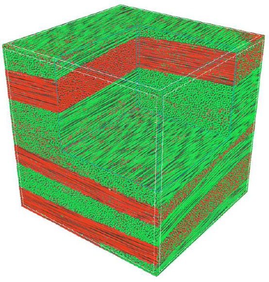
Bruker’s watershed algorithm is useful for studying grain-based materials, when a mass of closely packed particles can often appear as one single object rather than individual grains or fibres. This is relevant in a variety of fields, to reveal the properties of individual particles:
- Rocks and sediments in geology and geoscience
- Pellets
- Pharmaceutical particles
- Powders
- Pores
- Any grain-based material
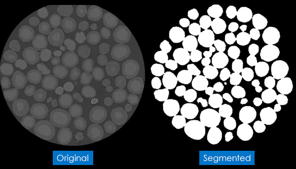
Usually, where particles or grains are stacked together, it’s difficult to study the properties of individual particles. Basic segmentation often selects the stack of particles all together as a single cluster. This makes it difficult to quantify them individually. Any pores, particles or fibres that are touching are usually counted as one single object, so you can’t measure them individually.
Watershed Separation
Bruker’s CTAn software includes a variety of despeckle and morphological tools. These include watershed separation, which is ideal for these granular samples.
The watershed separation algorithm divides connected objects into separate objects.
The name comes from watershed lines in geography, which divide landscapes and continents into individual basins. Mountain ranges are seen as separation lines (watersheds) between these regions.
The algorithm involves these steps:
- Segmentation
- Watershed separation:
– A distance map is calculated.
– (Local) minima are defined on the map.
– Individual objects are separated.
How it Works
1) Segmentation
The first step in performing a watershed separation is segmentation. There are several ways this can be carried out, including porosity analysis and adaptive thresholding.
Details about the various segmentation processes are described in method notes from Bruker (available to microtomography users through the Bruker Support portal: MN059, MN011 and MN020).
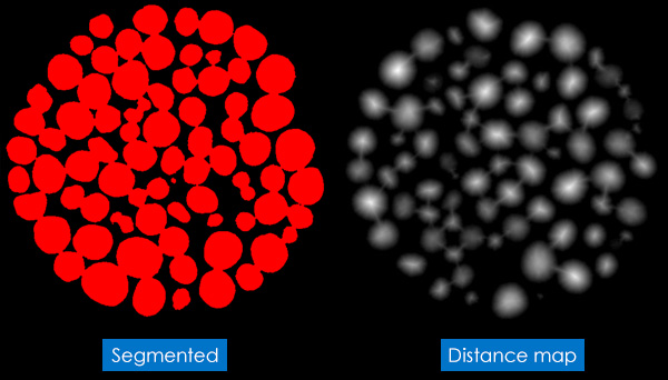
2) Distance mapping
The watershed separation algorithm automatically transforms the dataset into a distance map, like the one below.
It does this by calculating the shortest distance to the edge, for every point in each object. The grey values in the distance map indicate the distance to the edge at each point. This is performed automatically in the background.
3) Watershed separation
The distance map is then used as an input parameter, to separate the binary input dataset.
Each individual particle is separated from its neighbour by a thin black line. Where the grains are touching, this line could be just one voxel wide.
Adjust the Tolerance
With its default settings, the watershed algorithm is extremely sensitive to local minima. The tolerance value can be adjusted as you need to, to avoid over-separation.
Checking the Result
You can assign random colours to each particle, to quickly check the segmentation. This is a quick way of making sure that each grain has been defined correctly, and ensuring there’s no over-separation.

Analyse Grains/Particles Individually
You can then continue your analysis, and quantify the grains, particles or fibres individually:
- Density
- Morphometric parameters
- Volume
- Surface
- x, y, z location
- … and more
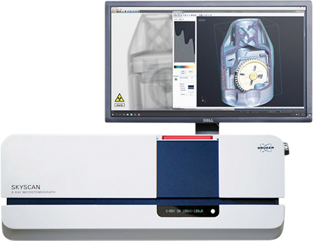
Bruker SkyScan Micro-CT
We offer the full range of Bruker SkyScan micro-CT scanners, which work with CTan software and the watershed algorithm. Just get in touch for advice about which would be best for your research.
You can view the complete range here.
Bruker SkyScan 1275
- Fast, benchtop scanner
- Automated scanning at the press of a button
- Self-optimising for the best results
- Extremely fast image reconstruction
Bruker SkyScan 2214
- Multi-scale X-ray nano-CT
- Widest range of sizes and resolutions
- World’s fastest image reconstruction
- Scan objects up to >300mm in diameter
More Information
Blue Scientific is the official distributor of Bruker SkyScan Micro-CT scanners in the UK and Nordic region (Finland, Norway, Denmark, Sweden and Iceland). We’re available to provide quotes and help with all your questions – just get in touch.
The separation process is described in more detail in Bruker’s Method Note 075 – Watershed Separation, which uses pharmaceutical particles as an example. This is available on request, or for micro-CT users via the Bruker Support website.